Chapter 3 Catalan and generating functions

Definition 3.1
Let $C (x) = \sum_{n \geq 0} c_{n} x^{n} = 1 + x + 2 x^{2} + 5 x^{3} + \dots$ denote the generating function of the Catalan numbers.

We can first deduce the recursive formula of the Catalan numbers $C (x) = 1 + x C (x)^{2} .$

We use the ordinary generating function for the Catalan numbers, we have $C (x) = \sum_{n \geq 0} c_{n} x^{n} = \sum_{n \geq 0} \sum_{k = 0}^{n - 1} c_{k} c_{n - 1 - k} x^{n}$ Since we know $C_{0} = 1$ , we have $\begin{aligned} C (x) & = \sum_{n \geq 0} \sum_{k = 0}^{n - 1} c_{k} c_{n - 1 - k} x^{n} \\ = 1 + \sum_{n \geq 1} \sum_{k = 0}^{n - 1} c_{k} c_{n - 1 - k} x^{n} \\ = 1 + x \sum_{n \geq 0} \sum_{k = 0}^{n} c_{k} c_{n - k} x^{n} \\ = 1 + x {(\sum_{n \geq 0} c_{n} x^{n})}^{2} \\ = 1 + x C (x)^{2} \end{aligned}$ Therefore, we got $C (x) = 1 + x C (x)^{2}$

Use the recursive formula ( $⋆$ ) to prove that $C (x)$ is a solution of the following equation of degree two:
$C (x) = 1 + x C (x)^{2} .$

From the equation $C (x) = 1 + x C (x)^{2}$ we have $C (x) = 1 + x C (x)^{2} \Rightarrow \frac{C (x) - 1}{x} = C (x)^{2}$ Then we try to prove the LHS equal to RHS.

For LHS we have $\begin{aligned} \frac{C (x) - 1}{x} & = \frac{\sum_{n \geq 1} c_{n} x^{n}}{x} \\ = \sum_{n \geq 0} c_{n + 1} x^{n} \end{aligned}$

For RHS, we apply we got $\begin{aligned} C (x)^{2} & = (\sum_{n \geq 0} c_{n} x^{n})^{2} \\ = \sum_{n \geq 0} (\sum_{k = 0}^{n} c_{k} c_{n - k}) x^{n} \\ = \sum_{n \geq 0} c_{n + 1} x^{n} (By Definition) \end{aligned}$

Therefore we have $C (x)^{2} = \sum_{n \geq 0} c_{n + 1} x^{n} = \frac{C (x) - 1}{x}$ Then we prove that $C (x)$ is a solution for the equation of $C (x) = 1 + x C (x)^{2}$

Deduce a formula for $C (x)$ and the radius of convergence.

Here we have the computation code in python

x = Symbol('x')
c = Symbol('c')
solution = solve(c - 1 - x * c**2, c)

# display the solution in latex
print("--------- Question 4.2 ----------")
print("The solution of the equation in is ")
display(solution[0]), display(solution[1])
print("The solution of the equation in Latex is ", (latex(solution[0])),
      latex(solution[1]))

We use sympy to solve the equation $C (x) = 1 + x C (x)^{2}$ and we get $C_{1} (x) = \frac{1 - \sqrt{1 - 4 x}}{2 x} and C_{2} (x) = \frac{1 + \sqrt{1 - 4 x}}{2 x}$ From the two possibilities, the $C_{1} (x)$ must be chosen because only the choice of the first gives $C_{0} = lim_{x \to 0} C_{1} (x) = 1$ Therefore we have $C (x) = \frac{1 - \sqrt{1 - 4 x}}{2 x}$

Then we compute the radius of convergence of $C (x)$ . For the definition of radius of convergence from Wiki page. We use the expression of $C (x)$ in power series that $C (x) = \frac{1 - \sqrt{1 - 4 x}}{2 x} = \sum_{n \geq 0} c_{n} x^{n}$ Base on [D’Alembert’s test], for radius of convergence $R$ we compute $lim_{n \to \infty} | \frac{c_{n + 1}}{c_{n}} | = ρ$ for $\sum_{n \geq 0} c_{n} x^{n}$ $\begin{aligned} ρ & = lim_{n \to \infty} | \frac{c_{n + 1}}{c_{n}} | \\ = lim_{n \to \infty} | \frac{\frac{1}{n + 2} (\binom{2 n + 2}{n + 2})}{\frac{1}{n + 1} (\binom{2 n}{n})} | \\ = lim_{n \to \infty} | \frac{4 n + 4}{n + 2} | \\ = lim_{n \to \infty} | 4 - \frac{4}{n + 2} | \\ = 4 \end{aligned}$ Since $ρ \neq 0$ , then we have the radius of convergence $R = \frac{1}{ρ} = \frac{1}{4}$

Compare the efficiency of different approaches.

knitr::include_graphics('static/pic3.png')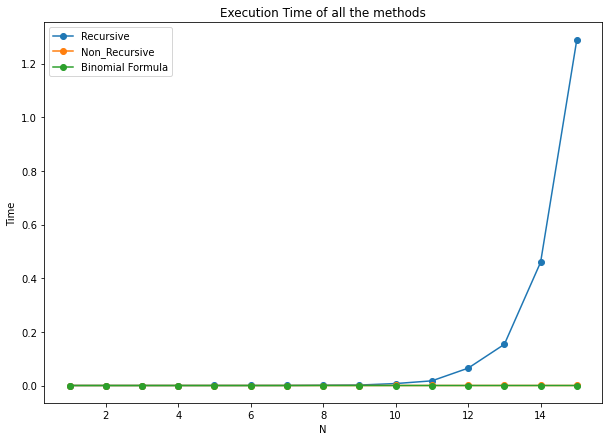

knitr::include_graphics('static/pic4.png')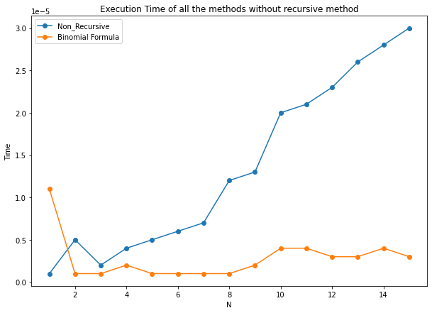

From the two graph we can see that the formula of $c_{n} = \frac{1}{n + 1} (\binom{2 n}{n})$ has the highest computation efficiency. However, the non-recursive method has more execution time than the method above, compare with recursive method the complexity is still much better since the execution time is in the level of $10^{- 5} s e c$ .

We can prove the expression of $c_{n} = \frac{1}{n + 1} (\binom{2 n}{n}) = \frac{(2 n)!}{(n + 1)! n!}$ with $C (x) = \frac{1 - \sqrt{1 - 4 x}}{2 x} = \sum_{n \geq 0} c_{n} x^{n}$

For power series we have $\sqrt{1 + y} = \sum_{n = 0}^{\infty} (\begin{matrix} \frac{1}{2} \\ n \end{matrix}) y^{n} = \sum_{n = 0}^{\infty} \frac{(- 1)^{n + 1}}{4^{n} (2 n - 1)} (\begin{matrix} 2 n \\ n \end{matrix}) y^{n}$ We denote that $y = - 4 x$ we got $\sqrt{1 - 4 x} = 1 - \sum_{n = 1}^{\infty} \frac{1}{2 n - 1} (\begin{matrix} 2 n \\ n \end{matrix}) x^{n}$ Therefore we got $C (x) = \frac{1 - \sqrt{1 - 4 x}}{2 x} = \sum_{n = 1}^{\infty} \frac{1}{2 (2 n - 1)} (\begin{matrix} 2 n \\ n \end{matrix}) x^{n - 1} = \sum_{n \geq 0} c_{n} x^{n}$ We can deduce that $c_{n} = \frac{1}{2 (2 n + 1)} (\binom{2 n + 2}{n + 1}) = \frac{1}{n + 1} (\binom{2 n}{n})$

3.1 Manipulate Generating Functions with SymPy

Definition 3.2
We work out with the example of $f (x) = \frac{1}{1 - 2 x} = 1 + 2 x + 4 x^{2} + 8 x^{3} + 16 x^{4} + \dots$ We first introduce variable $x$ and function $f$ as follows:

x=var('x')
f=(1/(1-2*x))

print('f = '+str(f))
print('series expansion of f at 0 and of order 10 is: '+str(f.series(x,0,10)))
display(f.series(x,0,10))

$1 + 2 x + 4 x^{2} + 8 x^{3} + 16 x^{4} + 32 x^{5} + 64 x^{6} + 128 x^{7} + 256 x^{8} + 512 x^{9} + O (x^{10})$

One can extract coefficient $n$ as follows: - $f$ has to be truncated at order $k$ (for some $k > n$ ) with f.series(x,0,k) - the $n$ -th coefficient is then extracted by f.coeff(x**n)

f_truncated = f.series(x,0,8)
print('Truncation of f is '+str(f_truncated))
n=6
nthcoefficient=f_truncated.coeff(x**n)
print(str(n)+'th coefficient is: '+str(nthcoefficient))
display(f_truncated)

$1 + 2 x + 4 x^{2} + 8 x^{3} + 16 x^{4} + 32 x^{5} + 64 x^{6} + 128 x^{7} + O (x^{8})$

Use SymPy to write another programm which computes the Catalan numbers using $C (x)$ , and compare the execution times with the functions of the first part of the Project.

# We compute C(x) with Taylor Expansion
x = var('x')
f = (1 - sqrt(1 - 4 * x)) / (2 * x)

def CatalanTaylorExpansion(n):
    return f.series(x, 0, n).coeff(x**(n - 1))
    
lis = [CatalanTaylorExpansion(i) for i in range(11)]
lis[1] = 1
print("The first ten Catalan numbers with Taylor Expansion are ", lis[1:])

The first ten Catalan numbers with Taylor Expansion are  [1, 1, 2, 5, 14, 42, 132, 429, 1430, 4862]

knitr::include_graphics('static/pic5.png')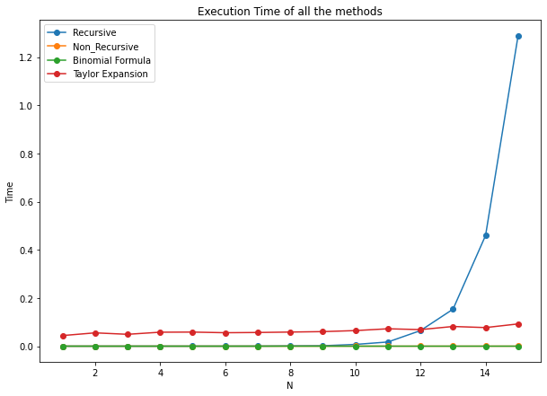

knitr::include_graphics('static/pic6.png')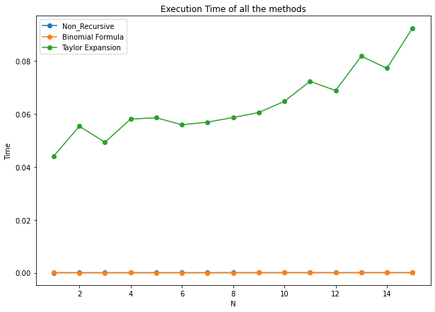

From the two graph we can see that the Taylor Expansion method is much faster than the recursive method but much slower than the method non-recursive and Binomial Formula.

3.2 Motzkin Numbers

Definition 3.3
The Motzkin numbers $m_{0}, m_{1}, m_{2}, \dots$ are similar to Catalan numbers and defined by $m_{0} = m_{1} = 1$ and for every $n \geq 2$ $m_{n} = m_{n - 1} + \sum_{k = 0}^{n - 2} m_{k} m_{n - 2 - k} .$

Find the generating function $M (x) = \sum_{n \geq 0} m_{n} x^{n}$ .
Compute the radius of convergence of $C$ and $M$ . Compare with numerical experiments: which sequence is growing fastest between $(c_{n})$ and $(m_{n})$ ?

We first try to simplify the motzkin numbers recurrence relation. We have $M (x) = \sum_{n \geq 0} m_{n} x^{n} = \sum_{n \geq 0} (m_{n - 1} + \sum_{k = 0}^{n - 2} m_{k} m_{n - 2 - k}) x^{n}$ Since we have $M_{0} = M_{1} = 1$ , therefore we have $\begin{aligned} M (x) & = \sum_{n \geq 0} (m_{n - 1} + \sum_{k = 0}^{n - 2} m_{k} m_{n - 2 - k}) x^{n} \\ = x \sum_{n \geq 0} m_{n - 1} x^{n - 1} + \sum_{n \geq 0} \sum_{k = 0}^{n - 2} m_{k} m_{n - 2 - k} x^{n} \\ = x M (x) + 1 + \sum_{n \geq 2} \sum_{k = 0}^{n - 2} m_{k} m_{n - 2 - k} x^{n} \\ = x M (x) + 1 + x^{2} \sum_{n \geq 0} \sum_{k = 0}^{n} m_{k} m_{n - k} x^{n} \\ = x M (x) + 1 + x^{2} (\sum_{n \geq 0} m_{n} x^{n})^{2} \\ = x M (x) + 1 + x^{2} M (x) \end{aligned}$

Therefore, we know that $M (x) = \sum_{n \geq 0} m_{n} x^{n}$ is a root for $x^{2} M^{2} + (x - 1) M + 1 = 0$ .

x = symbols('x')
M = symbols('M')
SeriesM = solve(x**2 * M**2 + x * M - M + 1, M)
print(SeriesM)
display(SeriesM[0])
display(SeriesM[1])

We use sympy to solve the equation we have $M_{1} (x) = \frac{1 - x - \sqrt{1 - 2 x - 3 x^{2}}}{2 x^{2}} M_{2} (x) = \frac{1 - x + \sqrt{1 - 2 x - 3 x^{2}}}{2 x^{2}}$ Since we know $M (0) = 1$ , therefore the only possible solution is $M (x) = \frac{1 - x - \sqrt{1 - 2 x - 3 x^{2}}}{2 x^{2}}$

# Implementation of the formula of Motzkin Numbers  
def MotzkinFormula(n):
    x = symbols('x')
    m= (1-x-sqrt(1-2*x-3*x**2))/(2*x**2)
    m_truncated = m.series(x,0,n+1)
    return m_truncated.coeff(x**n)
  
print("--------- Question 4.1.1.1 ----------")
lis = [MotzkinFormula(i) for i in range(11)]
lis[0] = 1
print("The first ten Motzkin numbers with Taylor Expansion are ", lis[1:])

--------- Question 4.1.1.1 ----------
The first ten Motzkin numbers with Taylor Expansion are  [1, 2, 4, 9, 21, 51, 127, 323, 835, 2188]

An integral representation of Motzkin numbers is given by $m_{n} = \frac{2}{π} \int_{0}^{π} \sin (x)^{2} (2 \cos (x) + 1)^{n} d x .$ They have the asymptotic behaviour $m_{n} \sim \frac{1}{2 \sqrt{π}} {(\frac{3}{n})}^{3 / 2} 3^{n}, n \to \infty$ Therefore, they have the same radius of convergence. We apply the similar method as Catalan number. Base on [D’Alembert’s test], for radius of convergence $R$ we compute $lim_{n \to \infty} | \frac{m_{n + 1}}{m_{n}} | = ρ$ for $\sum_{n \geq 0} m_{n} x^{n}$ $\begin{aligned} ρ & = lim_{n \to \infty} | \frac{m_{n + 1}}{m_{n}} | \\ = lim_{n \to \infty} | \frac{(\frac{3}{n + 1})^{\frac{3}{2}} 3^{n + 1}}{(\frac{3}{n})^{\frac{3}{2}} 3^{n}} | \\ = lim_{n \to \infty} | 3 (\frac{n}{n + 1})^{3 / 2} | \\ = 3 \end{aligned}$ Since $ρ \neq 0$ , then we have the radius of convergence $R = \frac{1}{ρ} = \frac{1}{3}$ .

Or we can illustrate in this way, from the definition of radius of convergence, we need to find an $R$ such that when $‖ x ‖ < R$ the series converges. Then we observe that radius shows when $1 - 2 R - 3 R^{2} = 0$ . Then we got $R = \frac{1}{3}$ or $r = - 1$ . Since when $x < 1$ , the function diverges, we can also get $R = \frac{1}{3}$

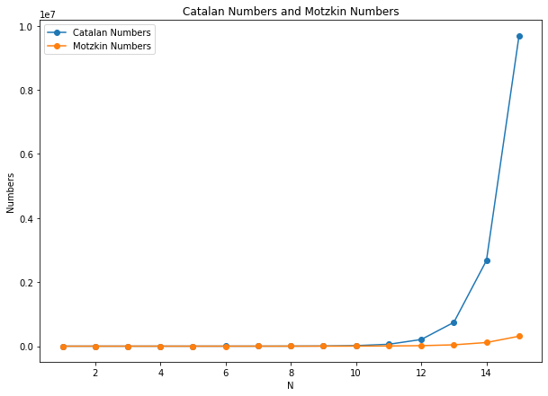
Then we can say the radius of convergence of $C$ is smaller than $M$ . Therefore the sequence of $c_{n}$ is growing faster than $m_{n}$ . We can also show this in the graph.

# plot the Catalan numbers and Motzkin numbers in the same graph
N = [i for i in range(1, 16)]
plt.figure(figsize=(10, 7))
lis_catalan = [CatalanNonRecursive(i) for i in range(1, 16)]
lis_motzkin = [MotzkinFormula(i) for i in range(1, 16)]
plt.plot(N, lis_catalan, 'o-', label='Catalan Numbers')
plt.plot(N, lis_motzkin, 'o-', label='Motzkin Numbers')
plt.legend()
plt.title("Catalan Numbers and Motzkin Numbers")
plt.xlabel("N")
plt.ylabel("Numbers")
plt.show()

knitr::include_graphics('static/pic7.png')